Phase Shifter
Full script
from functools import cached_property
from fnpcell import all as fp
from gpdk.technology import get_technology
from gpdk.technology.interfaces.wg import CoreCladdingWaveguideType
class PnPhaseShifterTemplate:
waveguide_type: CoreCladdingWaveguideType = fp.WaveguideTypeParam(type=CoreCladdingWaveguideType).as_field()
@cached_property
def curve_paint(self):
x_gap = 0.25
y_gap = 0.2
cont_w = 0.6
cont_h = 0.6
# m1_pin_w = 15
# m1_pin_h = 1.15
half_m1_h = 9.0
cladding_width = self.waveguide_type.cladding_width
y_offset = cladding_width / 2 + y_gap + 3 * cont_h / 2
array_h = cont_h * 3
p1_n1_h = array_h + y_gap + cladding_width / 2 + y_gap / 2
cont = fp.Device(
name="cont",
content=[
fp.el.Circle(radius=0.123, layer=TECH.LAYER.CONT_DRW),
fp.el.Rect(width=0.35, height=0.35, layer=TECH.LAYER.M1_DRW),
],
ports=[],
)
cont_array = (
cont.translated(cont_w / 2, cont_h / 2).new_array(cols=1, rows=3, col_width=cont_w, row_height=cont_h).translated(-1 * cont_w / 2, -3 * cont_h / 2)
)
print(cladding_width / 2 + y_gap + half_m1_h / 2)
return fp.el.CurvePaint.from_profile(
[
*self.waveguide_type.profile,
(
TECH.LAYER.M1_DRW,
[
(cladding_width / 2 + y_gap + half_m1_h / 2, [half_m1_h]),
(-cladding_width / 2 - y_gap - half_m1_h / 2, [half_m1_h]),
],
(0, 0),
),
(
TECH.LAYER.P_DRW,
[
(p1_n1_h / 2 + 0.525 / 2, [p1_n1_h - 0.525]),
],
(0, 0),
),
(
TECH.LAYER.P2_DRW,
[
(p1_n1_h / 2, [p1_n1_h]),
],
(0, 0),
),
(
TECH.LAYER.PP_DRW,
[
(y_offset, [array_h + y_gap * 2]),
],
(x_gap, x_gap),
),
(
TECH.LAYER.SIL_DRW,
[
(y_offset, [array_h]),
(-y_offset, [array_h]),
],
(0, 0),
),
(
TECH.LAYER.NP_DRW,
[
(-y_offset, [array_h + y_gap * 2]),
],
(x_gap, x_gap),
),
(
TECH.LAYER.N2_DRW,
[
(-p1_n1_h / 2, [p1_n1_h]),
],
(0, 0),
),
(
TECH.LAYER.N_DRW,
[
(-p1_n1_h / 2 - 0.525 / 2, [p1_n1_h - 0.525]),
],
(0, 0),
),
]
) + fp.el.CurvePaint.Composite(
[
fp.el.CurvePaint.PeriodicSampling(pattern=cont_array, period=cont_w, reserved_ends=(cont_w / 2, cont_w / 2), offset=y_offset),
fp.el.CurvePaint.PeriodicSampling(pattern=cont_array, period=cont_w, reserved_ends=(cont_w / 2, cont_w / 2), offset=-y_offset),
]
)
def __call__(self, curve: fp.ICurve):
return (
self.curve_paint(curve, offset=0, final_offset=0)
.with_ports(*self.waveguide_type.ports(curve, offset=0, final_offset=0))
.new_ref()
.with_name("pn_phase_shifter")
)
if __name__ == "__main__":
from pathlib import Path
gds_file = Path(__file__).parent / "local" / Path(__file__).with_suffix(".gds").name
library = fp.Library()
TECH = get_technology()
# =============================================================
template = PnPhaseShifterTemplate(waveguide_type=TECH.WG.SWG.C.WIRE)
ps = template(fp.g.Arc(radius=100, final_degrees=180))
library += ps
fp.export_gds(library, file=gds_file)
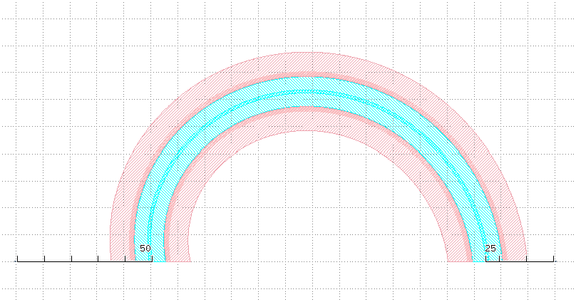
fp.plot(library)
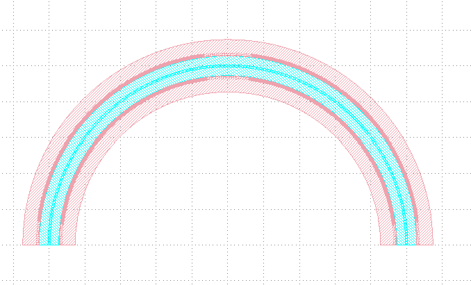
The following figure shows the GDS layout obtained after running the complete example script.
Segment Description
1. Import function module
from functools import cached_property
from fnpcell import all as fp
from gpdk.technology import get_technology
from gpdk.technology.interfaces.wg import CoreCladdingWaveguideType
2. Main function
if __name__ == "__main__":
  from pathlib import Path
  gds_file = Path(__file__).parent / "local" / Path(__file__).with_suffix(".gds").name
  library = fp.Library()
  TECH = get_technology()

  template = PnPhaseShifterTemplate(waveguide_type=TECH.WG.SWG.C.WIRE)        # Instantiate the defined class function
  ps = template(fp.g.Arc(radius=100, final_degrees=180))  # Define a circle curve with specified radius and angle and pass it to the class function and output the device
  library += ps       # Add the device to the library
  fp.export_gds(library, file=gds_file)       # Exporting GDS files
  fp.plot(library)    # Plot in PyCharm
3. Define function
First, some parameters of the device are defined
class PnPhaseShifterTemplate:
    waveguide_type: CoreCladdingWaveguideType = fp.WaveguideTypeParam(type=CoreCladdingWaveguideType).as_field()
    @cached_property
    def curve_paint(self):
        x_gap = 0.25
        y_gap = 0.2
        cont_w = 0.6
        cont_h = 0.6
        # m1_pin_w = 15
        # m1_pin_h = 1.15
        half_m1_h = 9.0
        cladding_width = self.waveguide_type.cladding_width
        y_offset = cladding_width / 2 + y_gap + 3 * cont_h / 2
        array_h = cont_h * 3
        p1_n1_h = array_h + y_gap + cladding_width / 2 + y_gap / 2
The below script is used to create individual base components.
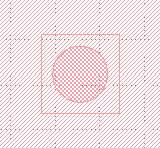
cont = fp.Device(
    name="cont",
    content=[
        fp.el.Circle(radius=0.123, layer=TECH.LAYER.CONT_DRW),  # Creates a circle of the specified radius on the corresponding layer
        fp.el.Rect(width=0.35, height=0.35, layer=TECH.LAYER.M1_DRW), # Create a rectangle with specified width and height values on the corresponding layer
    ],
    ports=[],   # No ports in this component
)
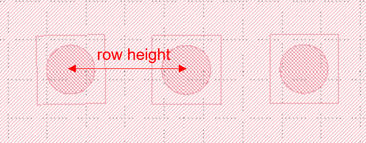
After having a single component, now create a set of array using the following procedure. In the script, the first translated function is to adjust the position of a single component, and then use the new_array function to create an array. col represents the number of rows; rows represents the number of columns; col_width represents the spacing between rows, and here is 1 row, so the value will not have a substantial impact; row_height is the column spacing, here is 3, adjusting the column spacing will change the horizontal distance between the center points of the array.
Finally, then use the translated function to position the entire array.
cont_array = (cont.translated(cont_w / 2, cont_h / 2).new_array(cols=1, rows=3, col_width=cont_w, row_height=cont_h).translated(-1 * cont_w / 2, -3 * cont_h / 2))
The following is the return part of the function, the original script defines a number of layer structure. However, for the convenience of explanation, here only the first layer acts as an example to explain the use of the function and parameters.
fp.el.CurvePaint.from_profile(profile, (layer, [A, B])) function is mainly based on the specified of a graphic profile to generate other graphic layer structures based on such profiles.
  return fp.el.CurvePaint.from_profile(
    [
        *self.waveguide_type.profile,   # Import the shape contour of the waveguide defined in the main function, and use it as a reference for all the graphs drawn later
        (
            TECH.LAYER.M1_DRW,
            [
                (cladding_width / 2 + y_gap + half_m1_h / 2, [half_m1_h]), # The value of t in [t] represents the total width of the layer; the value on the left represents the distance of the center of the layer from the center of the core layer; if positive, the radius decreases and negative increases

                (-cladding_width / 2 - y_gap - half_m1_h / 2, [half_m1_h]),
            ],
            (0, 0),  # This value is used for both ends of the extension, in front of the first port and at the end of the second port
        )
    ]
)
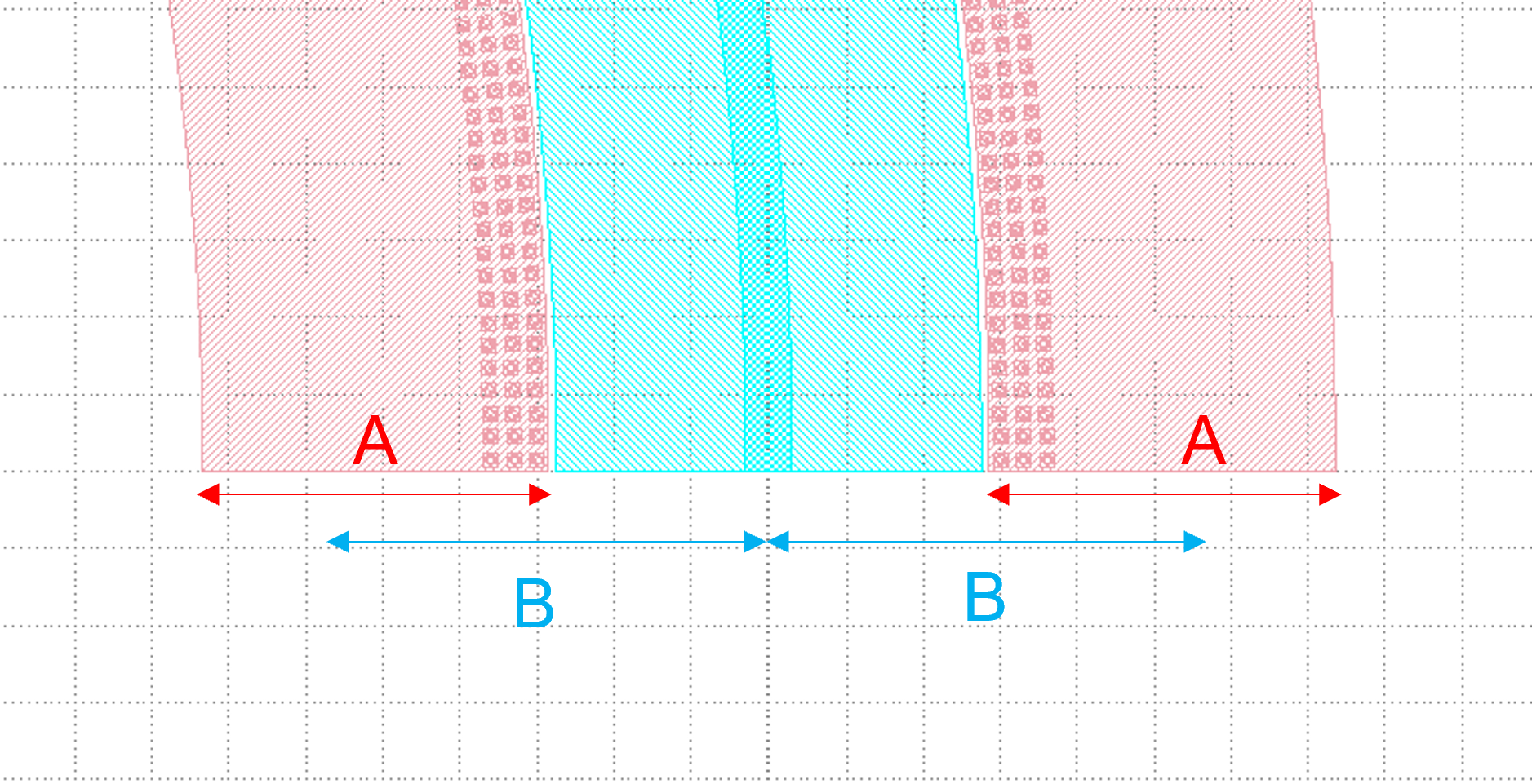
In the following figure, cladding_width / 2 + y_gap + half_m1_h / 2 is considered as value A and half_m1_h is considered as B. A is the M1_DRW layer width and B is the distance from the center of the layer to the center of the core layer.
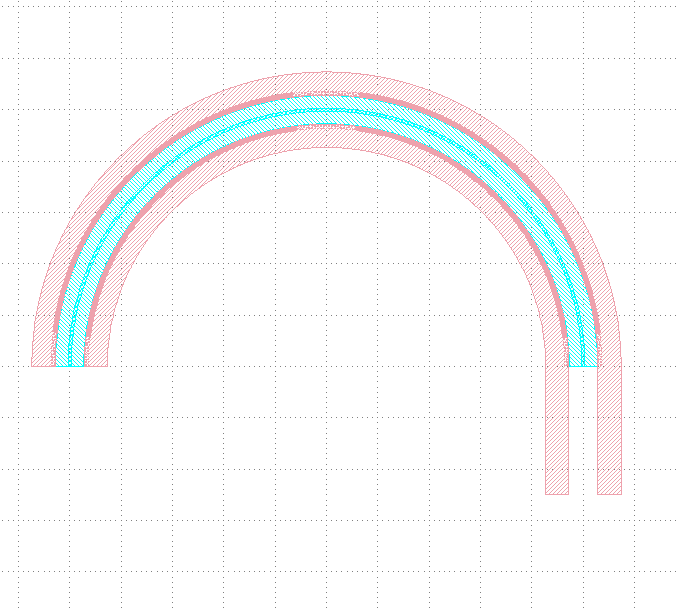
The following is a demonstration of the parameters to control the extension of the two ends. In the script for (0, 0), we first adjust the first 0 to 50, become (50, 0) and then run the script. From the figure below, you can see that the value on the left side of the brackets is used to control the extension of the starting end, and the extended section is a straight line not a circular arc.
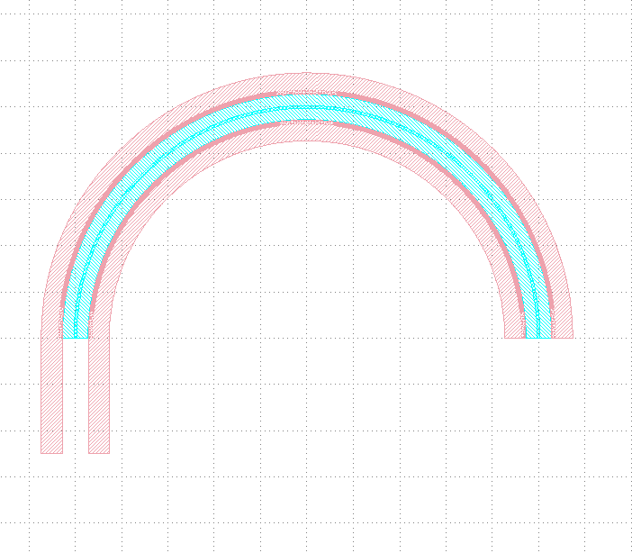
After changing (50,0) to (0,50) and running the script, you can see from the figure below that the right value controls the end extension, which also extends the line.
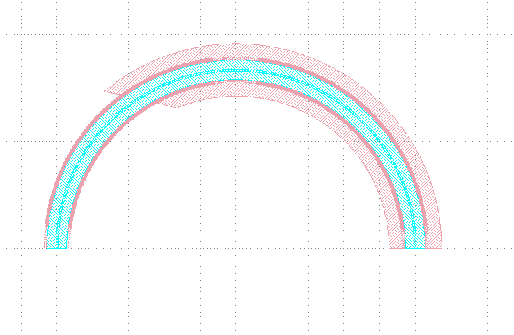
Now let’s change (0,50) to (0, -100) and run the script. As you can see from the graph, the end starts to recede and 100 indicates the length of the receding curve, which in this case is the arc length.
Then, we reset the above parameters and adjust the following part of the script, where the fp.el.CurvePaint.Composite() function is used to generate combined shapes; fp.el.CurvePaint.PeriodicSampling() is used to generate periodic shapes by sampling the shape of the curve for the period, where fp.el.CurvePaint. pattern is the original graph; period is the period of the shape, i.e., the spacing between the center points; reserved_ends=(a, b), a is the distance between the center point of the first array graph and the initial end, b is the distance between the center point of the last array graph and the end; offset is used to move the array graph according to the shape of the waveguide, similar to the increase and decrease of the radius of the circle, and its initial position is the center of the waveguide, negative means increasing the radius, positive means decreasing the radius.
  fp.el.CurvePaint.Composite(
    [
        fp.el.CurvePaint.PeriodicSampling(pattern=cont_array, period=cont_w, reserved_ends=(cont_w / 2, cont_w / 2), offset=y_offset),
        fp.el.CurvePaint.PeriodicSampling(pattern=cont_array, period=cont_w, reserved_ends=(cont_w / 2, cont_w / 2), offset=-y_offset),
    ]
)
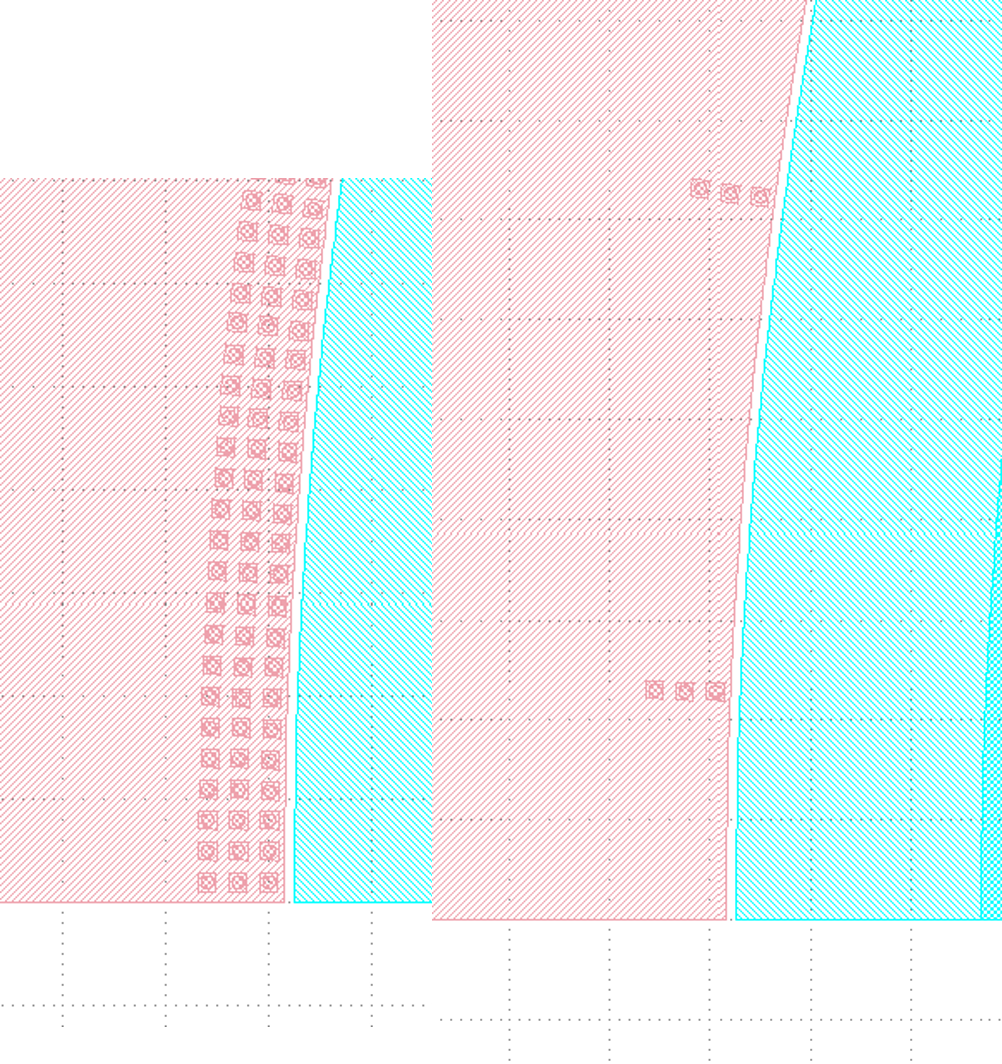
First we adjust the period parameter, run the original script, and get the following left figure array; then replace the value of 10 to run the script and get the following right figure, you can see that the spacing increased significantly.
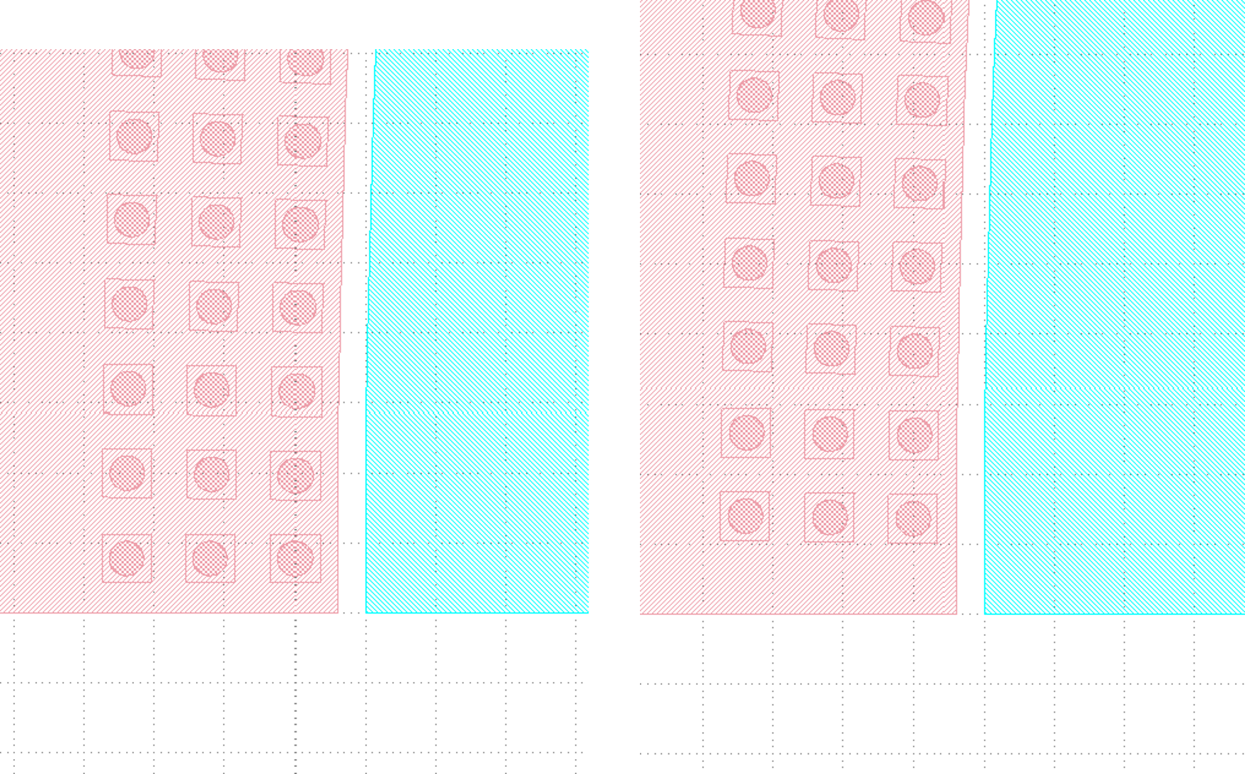
Then we adjust the reserved_ends parameter value, first after running the original script, we get the left graph below; change reseved_ends to (0, cont_w/2), we get the right graph below. After comparing the graphs, we can conclude that as the value increases, the curve where the center of each graph column is located will shorten by the corresponding value. While the value to the right of the reserved_ends bracket is responsible for controlling the end, the value to the left is responsible for controlling the initial end.
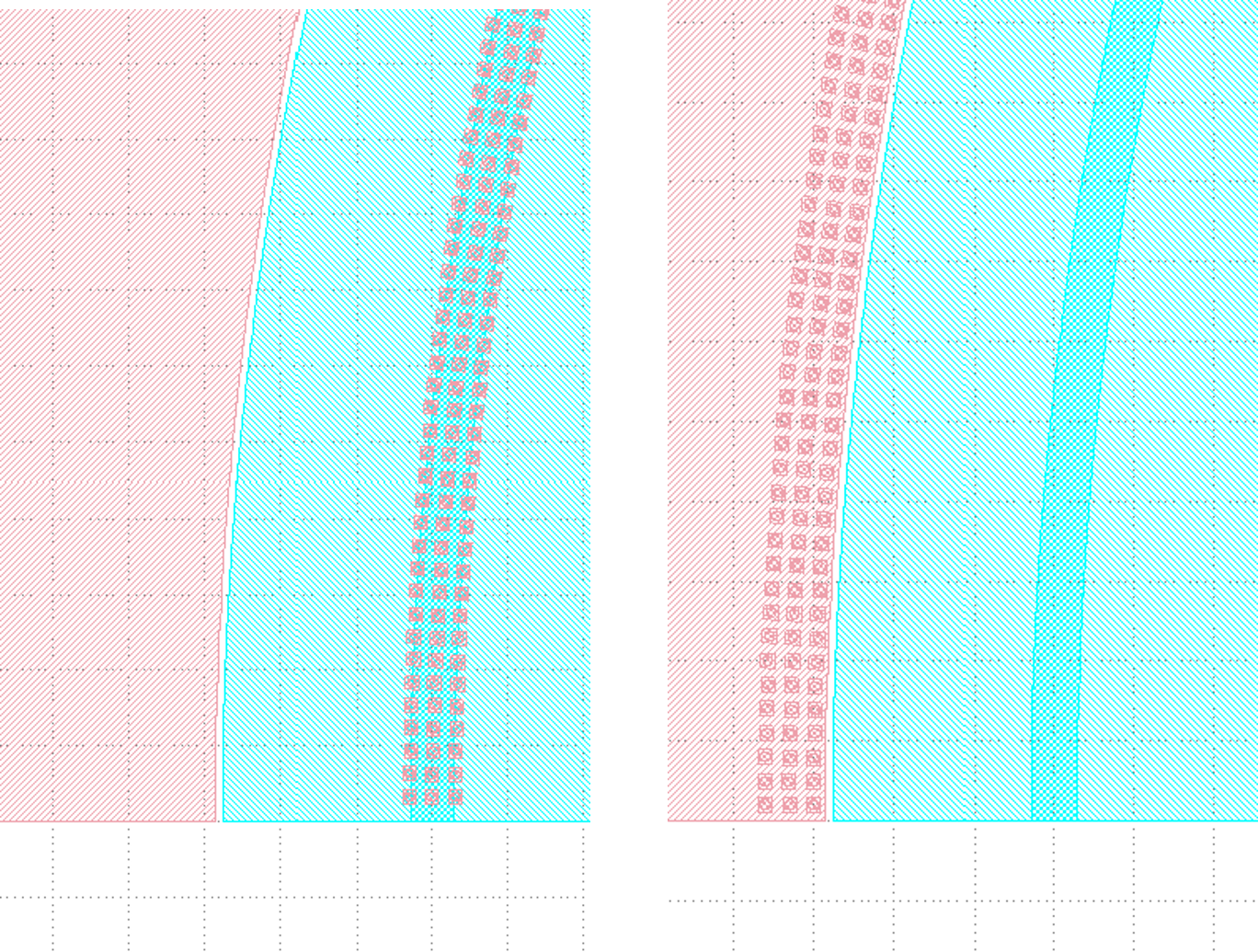
The following is a test of the offset. First, change the value of offset to 0 and run the script to get the left figure below; then reset the value of offset to y_offset and run the script to get the right figure below. From the figure below, we can compare that when the offset value represents the distance between the curve where the array is located and the waveguide curve, if it is positive, it moves to the left, if it is negative, it moves to the right.
The following part of the script explains the code through comments:
def __call__(self, curve: fp.ICurve):   # __call__ method is used for calling the simplified function "curve_paint"; blurs the distinction between object and function calls (improves code compatibility)
  return (
      self.curve_paint(curve, offset=0, final_offset=0)   # positive offset is to shift the op_0 port position to the negative direction of the x-axis; negative offset is to move to the x-positive direction; positive final_offset is to move the op_1 port to the x-positive direction.
      .with_ports(*self.waveguide_type.ports(curve, offset=0, final_offset=0))     # The position of the ports does not automatically follow the position of the waveguide, so the value of the correction has to be consistent with the waveguide.
      .new_ref()  # After testing, the new_ref() here has no real effect
      .with_name("pn_phase_shifter")  # Modify name
  )
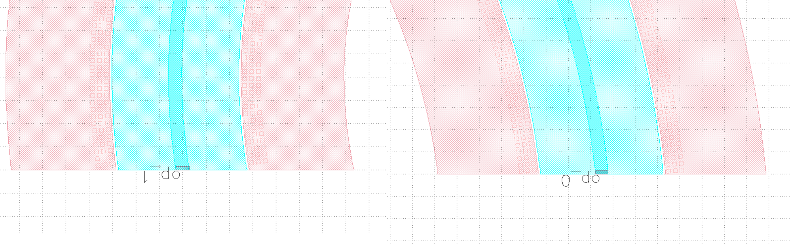
The following is a test of the offset and final_offset in the self.curve_paint function, setting their values to 25,50 respectively, and as you can see from the figure below, the end moves 50 in the positive direction of x and the initial end moves 25 in the negative direction of x.
In the above figure, although the waveguide has moved its position, the two port positions are still at the initial position. Now set the value of offset and final_offset in with_ports(*self.waveguide_type.ports(curve, offset=0, final_offset=0)) to 25,50 to match the corresponding position. As shown in the figure below, both op_1 and op_2 ports are already in the correct position, so the offset of ports needs to match with the offset value in curve_paint.